Example 01: Calculation of density currents in a tank
Purpose
To understand the basic operation of Nays2DV in iRIC by calculating the current field due to the density difference in a closed tank.
Creation of the calculation grid and setting the initial conditions
The grid for the Nays2DV model can be created only by using grid generator for Nays2DV.
Select[Grid] [Select Algorithm to Create Grid] then select [Grid Generator for Nays2DV] as shown in Figure 9.
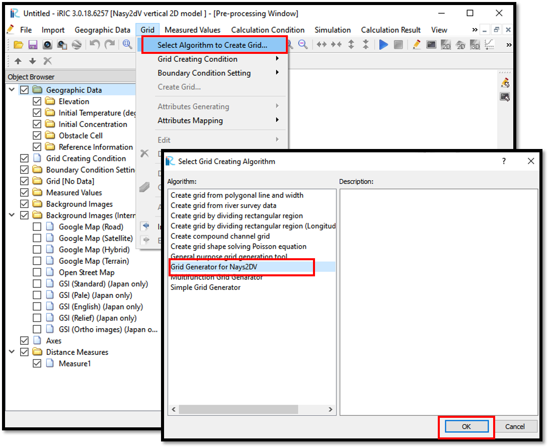
Figure 9 : Grid creation_1
Now the grid creation dialogue will appear as shown in Figure 10. Since the bottom profile data is not not available, select how to set longitudinal bed profile as automatically. If longitudinal bed profile data available, select manually and give the data for longitudinal bed profile.
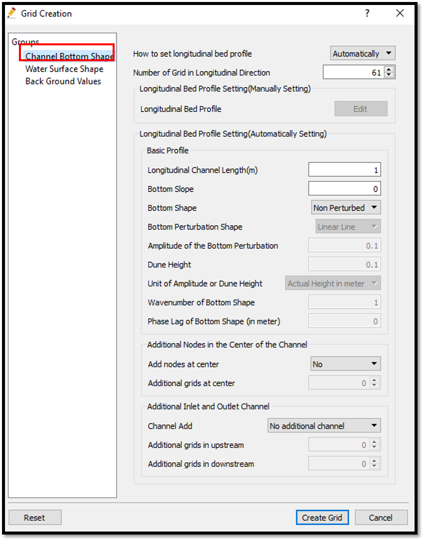
Figure 10 : Grid creation_2
Adjust the longitudinal details of the channel such as length and number of grids in x directions as required here. However, there is a maximum limit of the number of grids.
It is possible to adjust the bottom with a slope and perturb or non-perturb. This example a non perturbed bottom is used. See in the example with a cosine shaped bottom for a case with a perturb bottom and water surface.
If you have additional channels at upstream or downstream or both you can add here.
Water surface conditions and the number of grids in vertical direction can be given as shown in Figure 11.
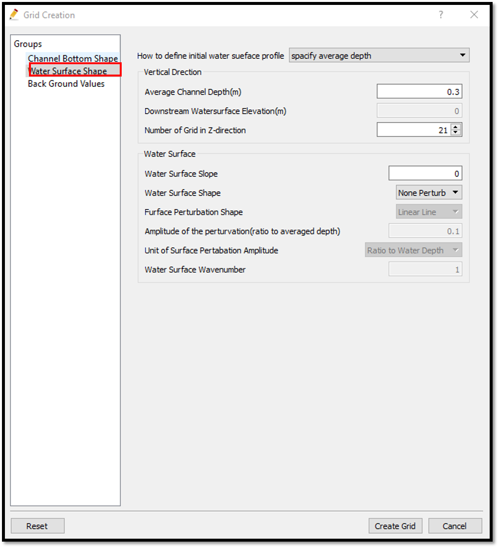
Figure 11 : Grid creation_3
Here you can adjust the water surface slope and shape perturb or non-perturb. If a flat one use non perturb and slope 0 as in this example. If you select perturb you can select either line, cosine or dune.
Background conditions of the creating grid can be given as shown in Figure 12.
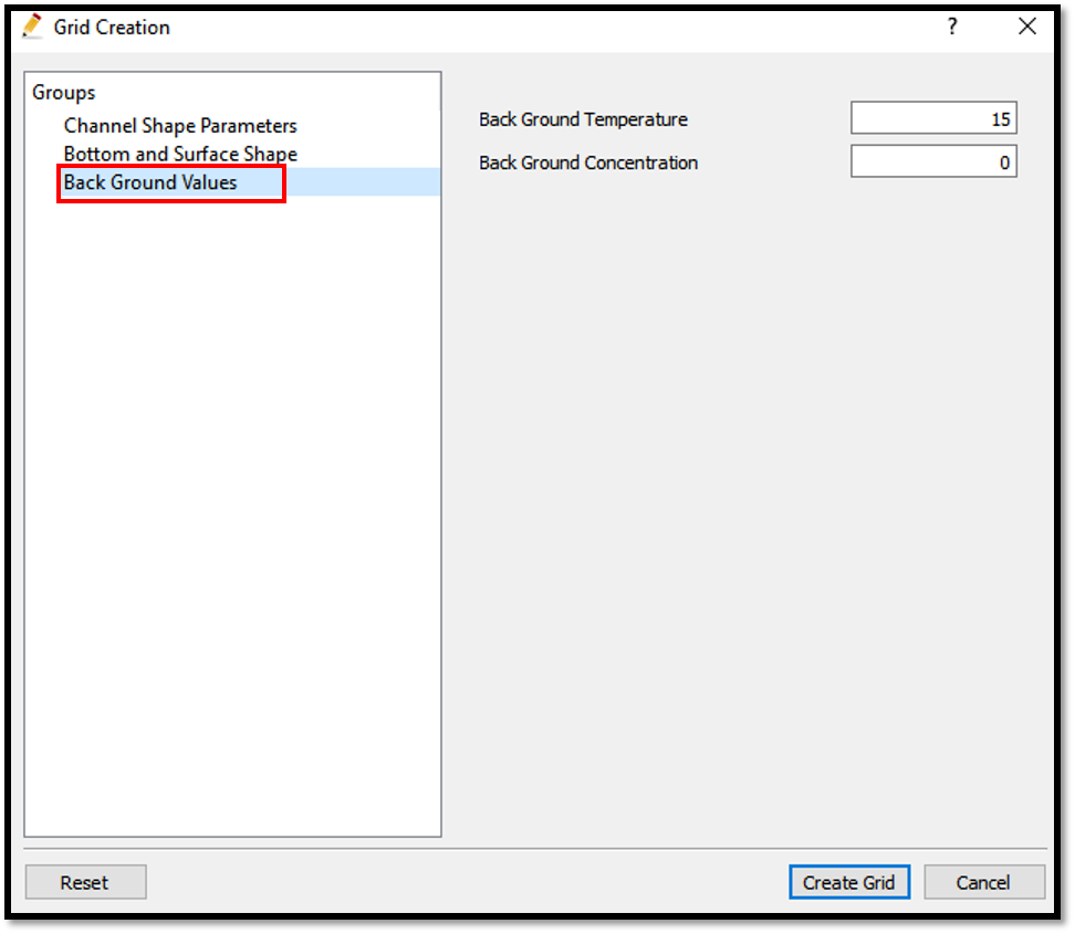
Figure 12 : Grid creation_4
Here give the values of the background temperature and concentration. This means the general condition of the calculation.
After setting up all the parameters create the grid. Then you will be asked to map the attributes or not. Select yes, as shown in Figure 13.
However, later if new conditions of temperature, concentration etc are added,should execute the attribute mapping again.
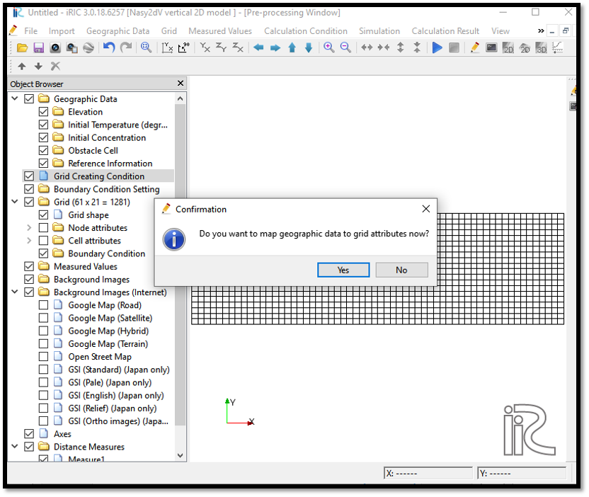
Figure 13 : Grid creation_5
The grid is created as shown in Figure 14.
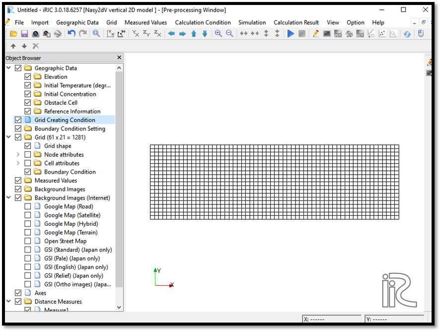
Figure 14 : Grid creation_6
Now, add a new concentration using a polygon as shown in Figure 15. [Initial Concentration] [Add] [Polygon] when the plus mark appear draw the polygon as required.
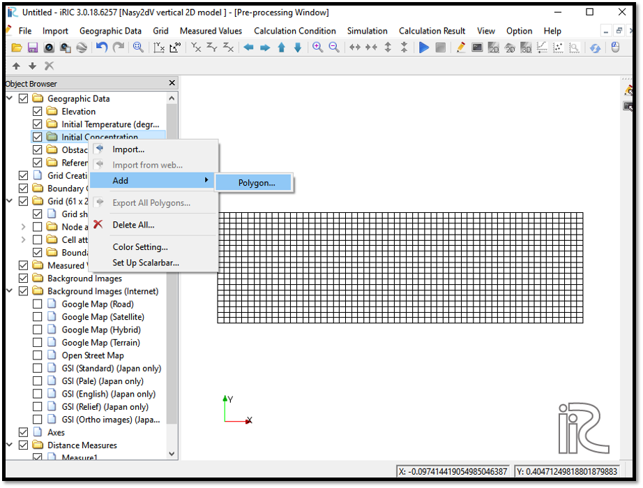
Figure 15 : Creating initial concentration polygon_1
After drawing the polygon, edit the values of the initial concentration of the drawn polygon as shown in Figure 16.
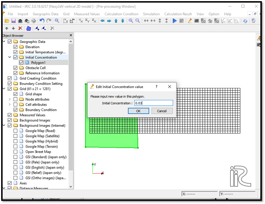
Figure 16 : Creating initial concentration polygon_2
In this example initial concentration is set to 0.03.
Now the new concentration needs to be mapped to the grids using, [Grid] [Attributes Mapping] and [Execute].
Then select the components needed to map. Select the parameters which changed the value. In this example it was initial concentration. Therefore, initial concentration is ticked as shown in Figure 17.
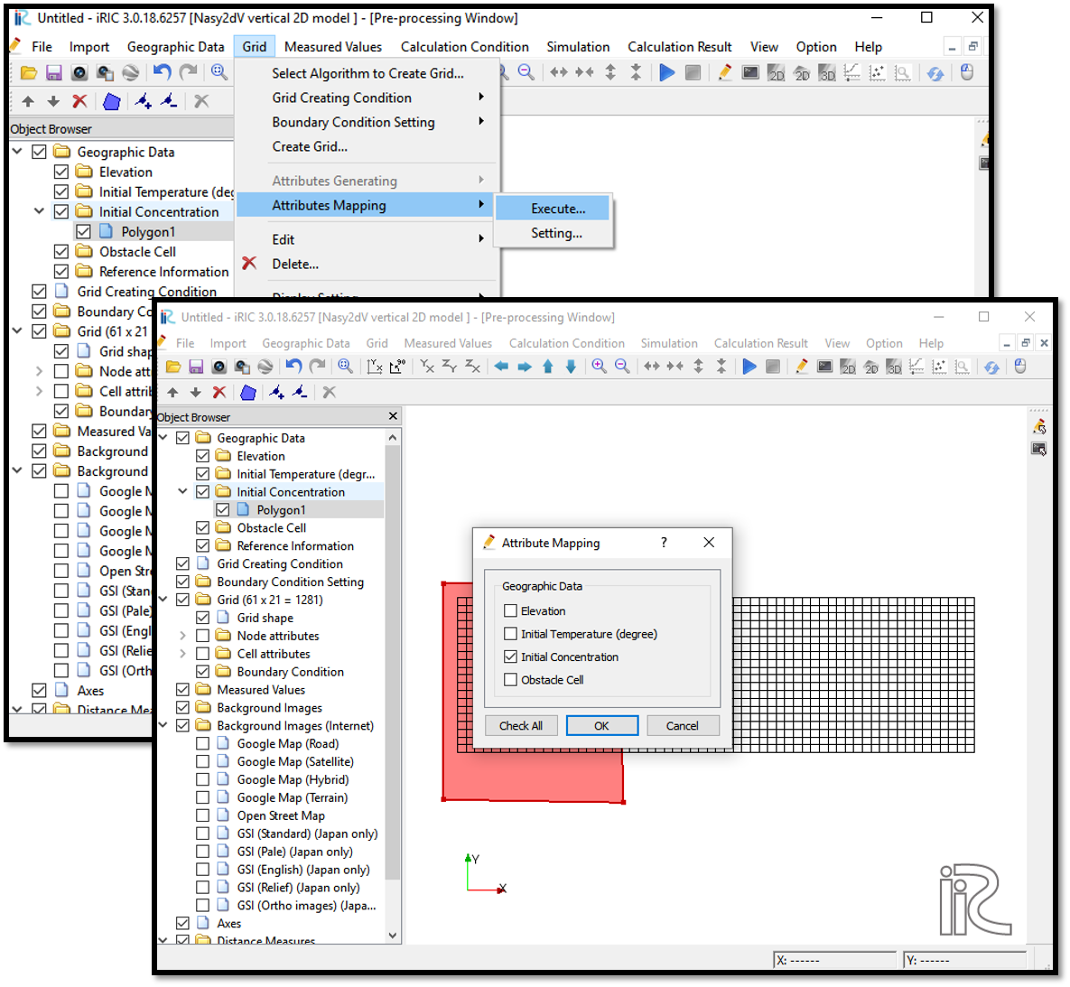
Figure 17 : Attributes mapping_1
The confirmation of mapping window will appear as shown in Figure 18.
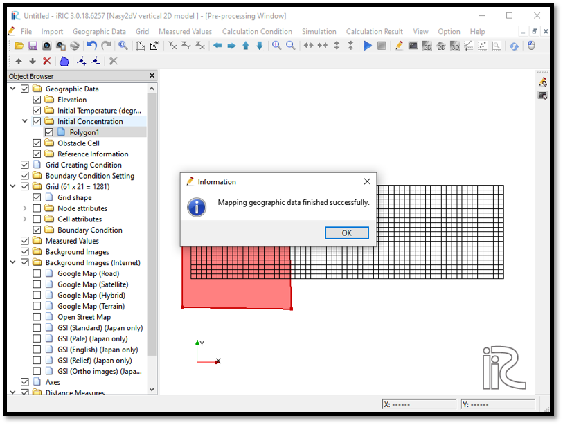
Figure 18 : Attributes mapping_2
After successful mapping of the attributes, it can be seen from the cell attributes and node attributes.
In this example check it in cell attributes.
In the [Object Browser] [Grid] [Cell Attributes] [Initial Concentration] as shown in Figure 19.
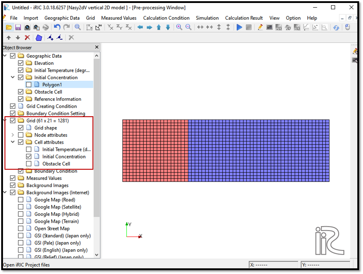
Figure 19 : Attributes mapping check
As shown in the figure, initial concentration is mapped properly.
Setting the calculation conditions and simulation
Next, calculation conditions need to be set.
For that, select [Calculation Conditions] and [Settings].
Then the calculation conditions window will open as shown in Figure 20. Input the values as shown in figure for computational parameters.
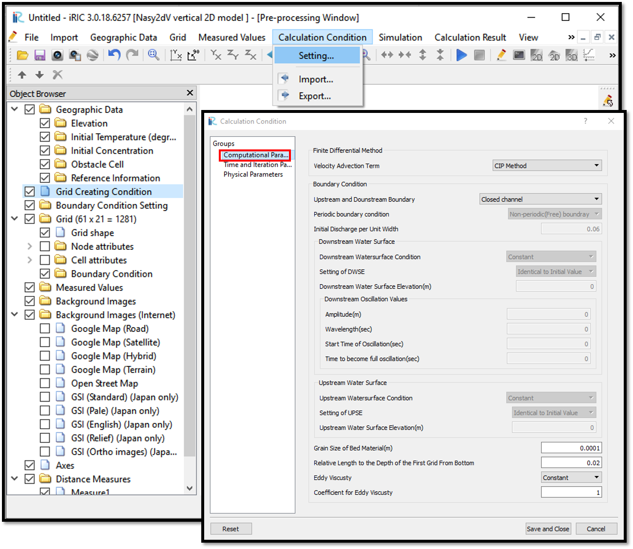
Figure 20 : Setting Calculation conditions_1
In this example, upstream and downstream boundary are closed boundary.
Then input parameters for time and iteration parameters as shown in Figure 21.
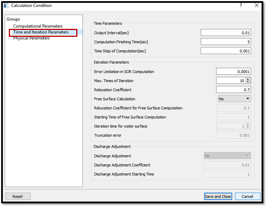
Figure 21 : Setting Calculation conditions_2
Time and iteration parameters are important for simulation stability.
Computational time step needs to be set considering the CFL condition according to the grid size.
If the computation fails at the initial stage, change the time step to a smaller value and try again.
Then adjust the physical parameters as shown in Figure 22.
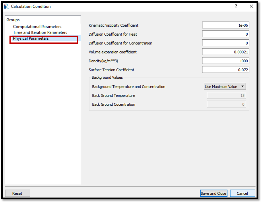
Figure 22 : Setting Calculation conditions_3
Physical parameters need to be adjusted according to the fluids used. In this example default values are used.
After setting all the calculation parameters, save and close the window.
Then save the project as density_currents.ipro and run the simulation with [Simulation] [Run] as shown in Figure 23.
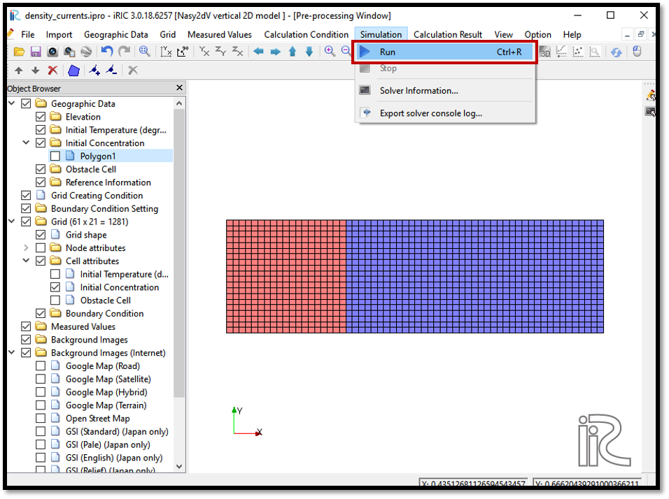
Figure 23 : Simulation_1
The simulation will end as shown in Figure 24.
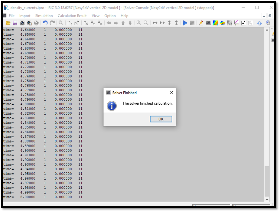
Figure 24 : Simulation_2
Visualization of results
After the computation is stopped, results can be viewed from [Calculation Results] [Open new 2D Post-Processing Window] as shown in Figure 25 or by clicking on 2D post-processing window icon.
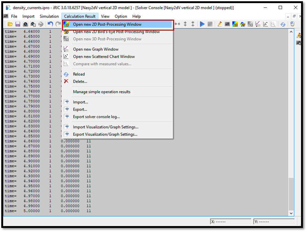
Figure 25 : Viewing results_1
The 2D post processing window will appear as shown in Figure 26
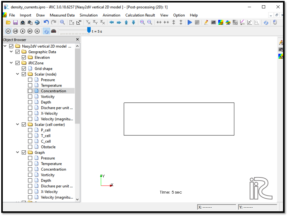
Figure 26 : Viewing results_2
In post processing window, the parameters need to be viewed can be selected in object browser. By adjusting the properties to desired scales, results can be visualized nicely. In this exmaple let’s visualize concentration and velocity vectors.
To visualize concentration,tick in object browser [iRIC Zone],[Scale],[Concentration]. Then right click on [Concetration] and select [Property]. The [Scaler Setting] window will appear as shown in Figure 27.
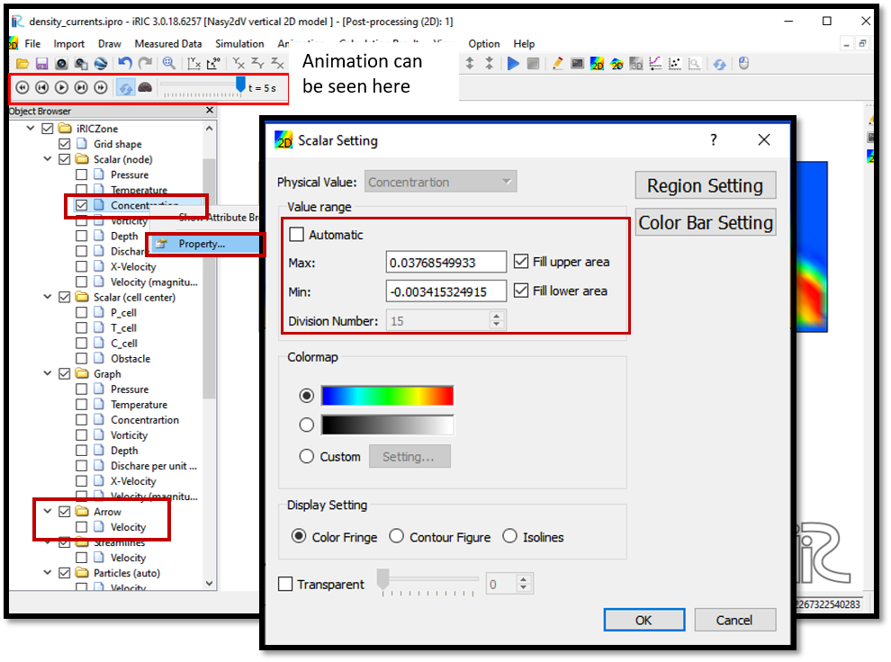
Figure 27 : Viewing results_3
As shown in the above figure, untick the automatic in [Value Range] and give themaximum and minimum values. In this example set minimum to 0 and maximum to 0.03. Tick on fill upper area and fill lower area.
To visualize velocity vectors together, tick on [Arrow] and [Velocity] both and right click on [Arrow], then select [Property].
[Arrow Setting] window will appear as shown in Figure 28.
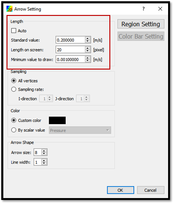
Figure 28 : Viewing results_4
Adjust the size of velocity vectors as shown in the figure.
Now the concentration and velocity vectors can be viewed as shown in Figure 29.

Figure 29 : Concentration and velocity vector plot
The animation of the movement can be viewed with animation buttons in top of the2D post-processing window.